Tensorflow for Statisticians (3)

Dealing with Survival Data

Last updated on Apr 17, 2022 4 min read

Another important type of data is the time-to-event structured survival data, which I worked on during my entire PhD study. Different from what we usually see, there may be censoring in survival data, which adds one more layer of complication to modeling.

The accelerated failure time (AFT) is a class of parametric models in describing the relationship between event times and covariates. It often assumes a parametric distribution for the logarithm of event times. The simplest model is to assume a lognormal distribution of event times, i.e.,

$\log(T) = \beta_0 + \beta_1 X_1 + \ldots + \beta_p X_p + \epsilon$;

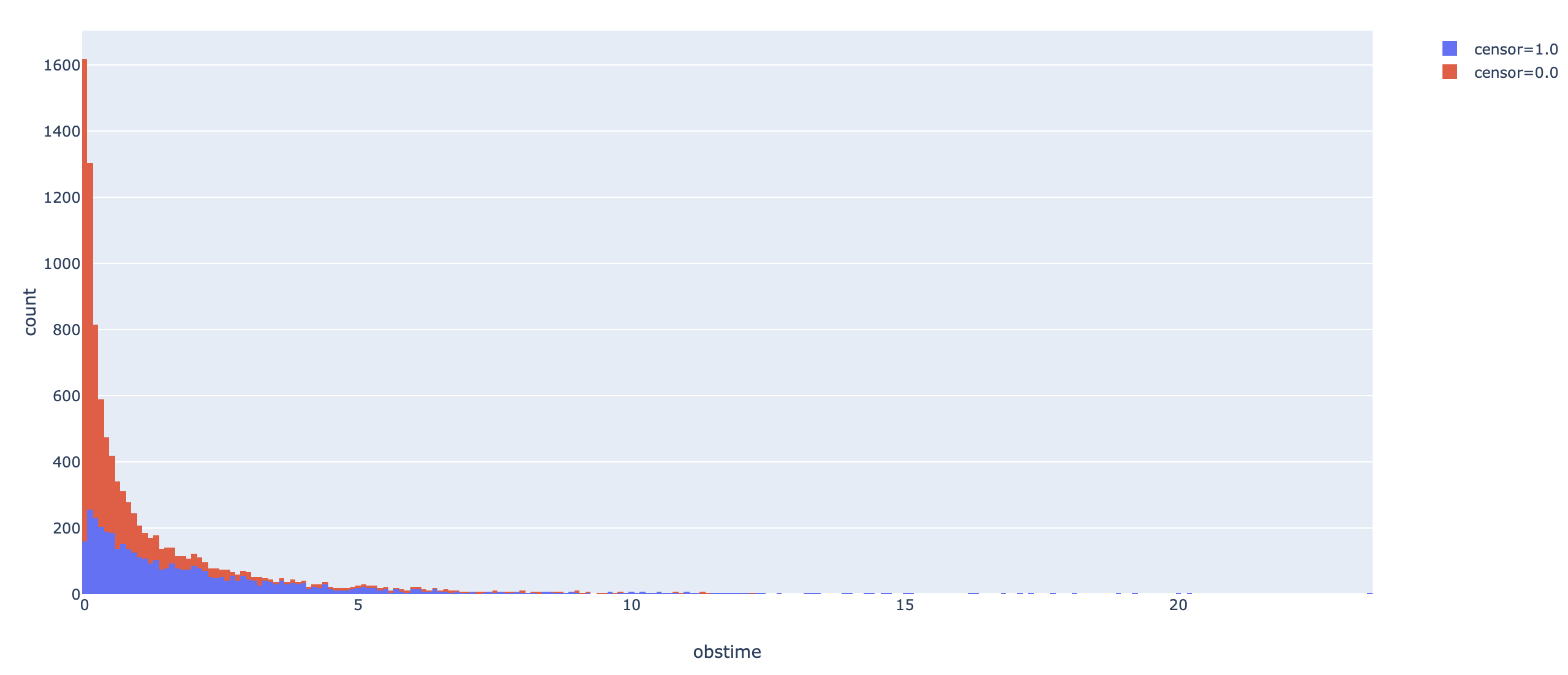
Conventionally, the censoring times are assumed to be independent from survival times, i.e., un-informative censoring is assumed.

Now we use a simple lognormal AFT model for illustration. First we simulate some data.

import tensorflow as tf
import tensorflow_probability as tfp
from tensorflow.keras import layers
tfd = tfp.distributions
import plotly as py
import plotly.express as px
import plotly.graph_objs as go
import numpy as np
import pandas as pd

## simulate normal covariates

def make_dataset(ndim, sd, nobs, seed):
    tf.compat.v1.random.set_random_seed(seed)
    X = tfd.Normal(0, 1).sample([nobs, ndim])
    pars = tfd.Uniform(0, 2).sample([ndim, 1])
    lp = tf.matmul(X, pars)
    Y = tfd.LogNormal(lp, sd).sample(1)
    Y = tf.reshape(Y, shape = [nobs])
    censortime = tfd.Exponential(rate = 1./3.).sample(nobs)
    obstime = tf.math.minimum(Y, censortime)
    censor = tf.math.greater(Y, censortime)
    censor = tf.cast(censor, dtype = tf.float32)
    return X, pars, obstime, censor

X, pars, Y, censor = make_dataset(10, 1, 10000, 1024)
dataa = pd.DataFrame({"obstime": Y, 
                      "censor": censor}, columns = ["obstime", "censor"])
fig = px.histogram(dataa, x="obstime", color="censor")
# fig.show()

Colored Histogram — A colored histogram of data generated by plotly; full code on GitHub.

The tricky thing here is to define a customized loss function. Usually it is rather easy as we only need to write out the log-likelihood function, but for survival data, it also depends on additional constants, which is the no-censor indicator, $\delta$, which equals 0 if an observation is censored, and 1 otherwise. The log-likelihood for the lognormal AFT model is given as:

$\sum_{i=1}^n \delta_i \log f(T_i) + (1-\delta_i) \log \left(1 - \Phi(\frac{\log(T_i) - \mu}{\sigma})\right)$,

where $f()$ is the pdf for lognormal distribution, with $\mu = X\beta$ and $\sigma=1$, and $\Phi()$ is the cdf for standard normal distribution. Now suppose we know the true $\sigma$, and only model the $\beta$. Our customized loss function can be written in the form of a closure. The `loss()` function inside the closure is the commonly seen form, but the `y_pred` is essentially the predicted $\mu$ in the lognormal distribution, not the predicted $y$ value. `loss1` calculates the log-likelihood when an observation is not censored, and `loss2` is the log-likelihood when it is censored. Finally we return the negative average log-likelihood, which is always positive, as the loss function, and minimize it numerically.

def loglike(censor):
    def loss(y_true, y_pred):
        loss1 = (- tf.math.log(y_true) - tf.pow(tf.math.log(y_true) - y_pred, 2) / 2.)
        loss2 = tf.math.log(1.- tfd.Normal(y_pred, 1,).cdf(tf.math.log(y_true)))
        return -tf.math.reduce_mean(censor * loss2 + (1.-censor) * loss1, axis = -1)
    return loss

model = tf.keras.Sequential()
model.add(layers.Dense(1, activation = "linear"))
model.compile(optimizer = tf.optimizers.Adam(0.01),
    loss = loglike(censor))
model.fit(X, Y, epochs = 100, batch_size = 50, verbose = False)

After 100 epochs, the model converged to have loss around 0.28. The model parameters and the true parameters are:

>>> model.layers[0].get_weights()[0]
# array([[0.96565   ],
#        [0.05977195],
#        [0.872731  ],
#        [0.5904592 ],
#        [0.31060567],
#        [0.69922787],
#        [0.8321791 ],
#        [0.11970102],
#        [0.6632817 ],
#        [0.58618313]], dtype=float32)
>>> pars
# <tf.Tensor: id=591325, shape=(10, 1), dtype=float32, numpy=
# array([[1.7620168 ],
#        [0.14598894],
#        [1.5785723 ],
#        [1.0458543 ],
#        [0.529089  ],
#        [1.1295629 ],
#        [1.4863789 ],
#        [0.15865707],
#        [1.1262481 ],
#        [1.0247502 ]], dtype=float32)>

This may seem off when we compare the estimation precision with linear regression. Using the survival package in R, the parameter estimate obtained is:

> round(fit$coefficients, 4)
#     X0     X1     X2     X3     X4     X5     X6     X7     X8     X9
# 0.2147 0.0089 0.1581 0.0910 0.0444 0.1416 0.1371 0.0113 0.1027 0.1072

This might be due to my poor data generation process. The code, however, is itself working!

In the future, I plan to write about:

enabling estimation of $\sigma$ in AFT models by customizing different activation functions for $\mu$ and $\sigma$
adding regularization to survival models
modeling more complicated distributions

technical tensorflow

Tensorflow for Statisticians (3)

Yishu Xue

Data Scientist / Coder / Novice Sprinter / Gym Enthusiast